Introduction to Reinforcement Learning
Resources:
Recap
- Generative AI Models and Applications:
- Text-to-Text and Text-to-Image models
- Architecture of Large Language Models (LLMs)
- Pre-training and fine-tuning of LLMs
- Reinforcement Learning with Human Feedback (RLHF) in fine-tuning LLMs
- Connection to this document’s focus:
- This document’s focus on Reinforcement Learning (RL) is broader than RLHF
- Will delve into underlying theory and diverse applications of RL
- How do you obtain your reward function in RLHF?
- Collect human feedback through comparisons of model outputs
- Human reviewers rank or compare outputs
- Preferences are used to train a reward model
- What do you use the reward function for?
- Fine-tune the LLM to generate preferred outputs
- Adjust model parameters to maximize the reward
- Encourage outputs that align with human preferences
Agenda Overview
- Introduction to Reinforcement Learning
- Motivation and key concepts
- Tools for experimenting with RL (e.g., Gymnasium)
- Key ingredients: States, Actions, Rewards
- Running Example: Blackjack
- Introduction and rules of the game
- Teaching an agent to play using RL
- Markov Decision Processes (MDPs)
- Modeling sequential decision-making problems
- Fundamental framework without learning algorithms
- Applying MDPs to Blackjack
- Deriving optimal strategies
- Challenges of explicit modeling
- Q-Learning
- Introduction to value-based RL methods
- Understanding the Q-Learning algorithm
- Applying Q-Learning to the Blackjack example
- Deep Q-Learning
- Extending Q-Learning to handle larger state spaces
- Conceptual differences from tabular Q-Learning
- Applications in complex environments (e.g., video games)
- Implementation details and code examples
Learning Objectives
- Understand Reinforcement Learning (RL):
- How RL differs from supervised and unsupervised learning
- The sequential and interactive nature of RL
- Comprehend Markov Decision Processes (MDPs):
- The modeling framework underlying RL methods
- Key components: states, actions, rewards, transition probabilities
- Learn Value-Based Methods:
- Grasp the concepts of Q-Learning
- Implement Q-Learning algorithms in code
- Apply Q-Learning to practical problems like Blackjack
- Explore Deep Q-Learning:
- Understand how Deep Q-Learning extends Q-Learning
- Address problems with large or continuous state spaces
- See real-world applications and code implementations
Reinforcement Learning Introduction
Thought Exercise: Dice Game
The considerations to make when thinking about a strategy to play this game are similar to what gets modeled in Markov Decision Processes.
- Game Rules:
- Roll a six-sided die
- If it lands on 1:
- If it lands on 2-6:
- Choose to stop and receive N dollars (N = die number)
- Or choose to roll again
- Objective: Maximize winnings by deciding when to stop
- Strategic Considerations:
- Risk vs. Reward:
- Higher numbers offer better immediate rewards
- Rolling again risks landing on 1 and losing all winnings
- Decision-Making Over Time:
- Multiple opportunities to make choices
- Uncertainty about future die rolls
- Questions to Ponder:
- When is it optimal to stop?
- How does the probability of future outcomes affect current decisions?
Applications of Reinforcement Learning
- Robotics:
- Teaching robots to perform tasks through interaction
- Example: Quadruped robot learning to walk
- Starts with no predefined walking strategy
- Learns by trial and error, receiving rewards for desirable behaviors
- Adapts to disturbances (e.g., being pushed)
- Games:
- Learning to play board games (e.g., Backgammon)
- RL agents can surpass human expertise
- Influence on human strategies and game understanding
- Video games and complex environments
- Other Fields:
- Finance: Portfolio management, trading strategies
- Public Policy: Potential applications with simulation models
- Challenges due to delayed feedback and complexity
Key Concepts of Reinforcement Learning
- Agent-Environment Interaction:
- Agent: Learns and makes decisions
- Environment: The system the agent interacts with
- Feedback Loop:
- Agent takes an action
- Environment provides state and reward
- Agent updates its strategy based on feedback
- Components:
- State: Observation of the environment at a given time
- Action: Decision made by the agent
- Reward: Feedback signal indicating success or failure
- Goal:
- Learn a policy that maximizes cumulative rewards over time
Differences from Other Machine Learning Paradigms
- Supervised Learning:
- Learning from labeled data
- Predicting outputs from inputs
- Unsupervised Learning:
- Finding patterns in unlabeled data
- Clustering, dimensionality reduction
- Reinforcement Learning:
- Learning from interactions with the environment
- No explicit labeled data
- Focus on sequential decision-making and long-term rewards
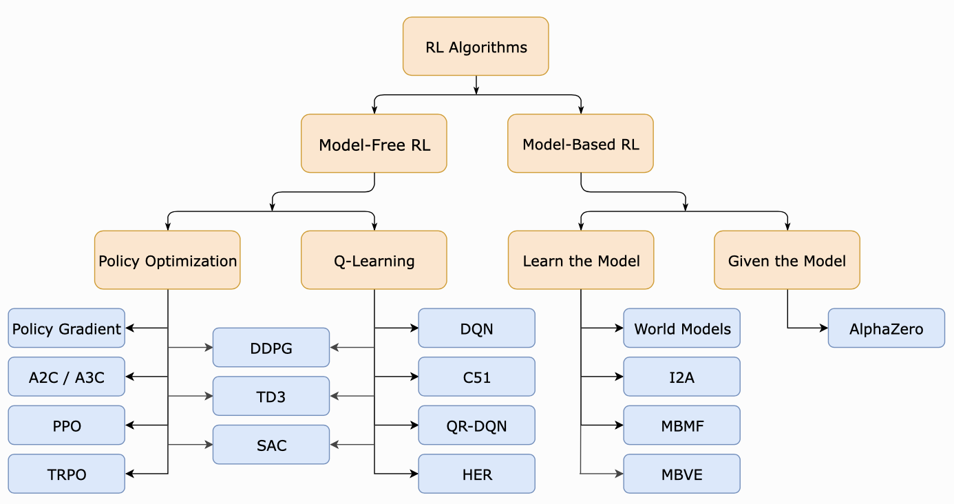
Types of Reinforcement Learning Methods

- Model-Free Methods:
- Do not require a model of the environment
- Value-Based Methods: (Covered in this document)
- Estimate the value of actions
- Example: Q-Learning
- Policy-Based Methods: (Covered in RL Part 2)
- Directly optimize the policy function
- Model-Based Methods:
- Build a model of the environment’s dynamics
- Plan actions using the model
- Multi-Agent RL:
- Multiple agents learning and interacting
- Coordination and competition dynamics
- Overview:
- A toolkit for developing and comparing RL algorithms
- Provides a variety of environments with a consistent interface
- Successor to OpenAI Gym, now maintained by Farama
- Key Features:
- Common Interface:
- Easy to switch between different environments
- Simplifies testing algorithms across multiple settings
- Environment Categories:
- Classic Control: Simple physical systems (e.g., CartPole)
- Robotics: Complex simulations with multiple degrees of freedom
- Games: Simple games like Blackjack, Atari 2600 games
- Custom Environments: Users can create their own
- Example Environments:
- CartPole: Balance a pole on a moving cart
- Lunar Lander: Control a lander to touch down safely
- Blackjack: Card game simulation
- Atari Games: Classic games for complex RL tasks
- Basic Usage:
import gymnasium as gym
env = gym.make("LunarLander-v2", render_mode="human")
observation, info = env.reset(seed=42)
for _ in range(1000):
    action = env.action_space.sample() # this is where you would insert your policy
    observation, reward, terminated, truncated, info = env.step(action)

    if terminated or truncated:
        observation, info = env.reset()

env.close()
Running Example: Blackjack Environment
Blackjack Rules Recap
- Objective: Get a hand total as close to 21 as possible without exceeding it
- Gameplay:
- Player and Dealer: Each starts with two cards
- Card Values:
- Number cards: Face value (2-10)
- Face cards (J, Q, K): 10
- Ace: 1 or 11 (player’s choice)
- Player Actions:
- Hit: Take another card
- Stand: End turn with current hand
- Dealer Actions:
- Reveals one card initially
- Plays after the player stands
- Must hit until reaching a certain total (usually 17)
- Winning Conditions:
- Player’s hand total is higher than dealer’s without exceeding 21
- Dealer busts (exceeds 21), player doesn’t
Blackjack Environment Code
Gymnasium (formerly OpenAI Gym) is a popular toolkit for testing reinforcement learning algorithms. It provides simulation environments for a variety of RL tasks and a simple common interface for interacting the environments. In this notebook we will work with the Blackjack environment, which plays the popular casino game Blackjack. We will introduce the basic mechanics of the Gymnasium Blackjack environment by manually playing a hand.
# First we will install the Gymnasium package
# !pip install gymnasium

import gymnasium as gym
import torch
import torch.nn.functional as F

import random
import numpy as np
from IPython import display
from collections import deque, OrderedDict
import matplotlib.pyplot as plt

"""
Here we interact directly with the Blackjack environment to get
a feel for how it works
"""

# Create the environment
env = gym.make("Blackjack-v1", render_mode="rgb_array")

# Deal the cards / sample an initial state
obs = env.reset()[0]

# Render a visualization in the notebook
plt.imshow(env.render())
plt.show()
print(obs)

# Loop as long as the hand has not finished
done = False
while not done:

    # Choose an action: 1 is hit, 0 is stand
    action = int(input("Hit (1) / Stand (0): "))

    # Provide the action to the environment and update the game state
    # The environment returns three values that we care about:
    # - obs: The current state (or "observation", equivalent in this case)
    # - reward: The reward earned in the current step
    # - done: A boolean indicating whether the hand is done or in-progress
    obs, reward, done, truncated, info = env.step(action)

    # Render the updated state in the notebook
    display.clear_output(wait=True)
    plt.imshow(env.render())
    plt.show()
    print(obs, reward, done, truncated, info)

env.close()
A few notes to take away:
- We first created our environment with
gym.make.
- We initialize the environment (deal the cards, in this case) with
env.reset().
- Initializing the environment returns a game state (which we assign to the variable
obs). The state is a tuple containing the information (player_current_total, dealer_card, usable_ace).
- We iterate over turns until the game terminates. In each turn we choose an
action (“hit” or “stay”).
- When we provide our selected action to the environment,
env.step updates the state of the environment.
env.step also provides a reward in each step. For this environment, reward is 1.0 if we win the hand, -1.0 if we lose the hand, and 0.0 otherwise.
Interacting with the Blackjack Environment
- State Representation:
- Player’s Current Hand Total
- Dealer’s Visible Card
- Usable Ace Indicator: Whether the player has an ace counted as 11
- Actions:
- Hit (1): Take another card
- Stand (0): Keep current hand
- Rewards:
- +1: Player wins
- 0: Draw
- -1: Player loses
Implementing a Simple Policy
The aim of Reinforcement Learning is to learn effective strategies for automatically selecting an action in each time period based on the current state of the environment. Rules for selecting an action based on the current state are known as policies. Here, we will manually create a simple heuristic policy and demonstrate how it controls the environment. We will evaluate this policy by playing 50,000 hands of Blackjack and counting the fraction of hands won under this policy.
def simple_policy(state):
    """
    This simple policy always hits (draws another card) if the total value of
    the player's hand is less than 17, and stays if the value of the player's
    hand is greater than or equal to 17.
    """

    # The first component of the state is the player's hand
    # If that is less than 17, hit. Otherwise stay.
    if state[0] < 17:
        return 1
    else:
        return 0
Running Simulations
- Purpose: Evaluate the effectiveness of the policy
- Simulation Steps:
- Initialize Environment:
- Loop Over Episodes:
- Apply policy to decide actions
- Collect rewards and track outcomes
- Collect Statistics:
- Calculate win rate
- Analyze policy performance
- Sample Results:
- Simple policy might achieve a win rate around 41%
Key Elements in Reinforcement Learning
States
- Definition: Information that captures the current situation
- Characteristics:
- Must include all relevant details to make optimal decisions
- Should summarize past and present information necessary for future predictions
- In Blackjack:
- Hand Total: Sum of card values
- Dealer’s Visible Card: Provides context on dealer’s potential hand
- Usable Ace: Flexibility in counting an ace as 1 or 11
Actions
- Definition:
- The decisions an agent can make at each time step.
- In Blackjack:
- Hit: Take another card.
- Stand: Stop taking cards.
- Properties:
- Actions influence the environment.
- Actions can change the state and affect future rewards.
- Actions are taken sequentially over time.
Rewards
- Definition:
- Feedback received from the environment after taking an action.
- In Blackjack:
- Win: Receive a reward of +1.
- Lose: Receive a reward of -1.
- Game in Progress: Receive a reward of 0.
- Goal:
- Select actions that move towards states likely to yield positive rewards.
- Must consider future rewards, not just immediate ones.
State Transitions
- Definition:
- The probability of moving from one state to another after taking an action.
- Importance:
- Determines how actions lead to new states.
- Influenced by both the current state and the action taken.
- In Blackjack:
- Example:
- Current State: (14, 10, 0)
- Player’s hand total: 14
- Dealer’s visible card: 10
- No usable ace
- Hit Action:
- Possible next states:
- (16, 10, 0)
- (17, 10, 0)
- (19, 10, 0)
- Each transition has a probability based on the card drawn.
- Stand Action:
- Remain in current hand total.
- Dealer plays, resulting in a win or loss.
- Transition to a terminal state with a reward of +1 or -1.
- Modeling Challenges:
- Requires explicit calculation of transition probabilities.
- Complex due to the randomness in the environment.
- Learning Algorithms:
- Implicitly learn state transitions through interaction.
- Do not require explicit modeling of transition probabilities.
Generalizing to Multi-Stage Decision Problems
- Common Characteristics:
- Sequential Decisions:
- Actions are taken over multiple time steps.
- State Information:
- Decisions are based on the current state.
- Uncertainty:
- Outcomes are not deterministic.
- Balancing Rewards:
- Trade-off between immediate and future rewards.
- Need for a Mathematical Framework:
- Markov Decision Processes (MDPs):
- Provide a structured way to model these problems.
- Capture states, actions, rewards, and transitions.
Markov Decision Processes (MDPs)
Definition
- Components:
- Finite Set of States (S):
- All possible states an agent can be in.
- In Blackjack: All combinations of hand totals, dealer’s visible card, and usable ace status.
- Finite Set of Actions (A):
- All possible actions available to the agent.
- In Blackjack: Hit or Stand.
- Reward Function (R):
- Maps state-action-next state to rewards.
- $ R(s, a, s’) $: Reward received when transitioning from state $ s $ to state $ s’ $ using action $ a $.
- State Transition Probabilities (P):
- $ P(s’ | s, a) $: Probability of transitioning to state $ s’ $ from state $ s $ using action $ a $.
- Initial State Distribution (optional):
- Distribution over starting states.
- Often not crucial for solving the MDP.
- Goal:
- Find a policy that maximizes the expected cumulative reward over time.
Time Horizons in MDPs
Episodic Tasks
- Characteristics:
- Have a clear start and end.
- Terminal States:
- States where the episode ends.
- Finite Time Horizon:
- Accumulate rewards over a limited number of steps.
- Example:
- Blackjack:
- Game starts when cards are dealt.
- Ends when player wins or loses.
Continuing Tasks
- Characteristics:
- Run indefinitely without a terminal state.
- Infinite Time Horizon:
- Accumulate rewards over an infinite sequence.
- Example:
- Robotics Control:
- A robot performing tasks continuously.
Modeling Episodic Tasks as Continuing Tasks
- Technique:
- Introduce Terminal (Absorbing) States:
- Once entered, the agent remains there indefinitely.
- Transition back to the same state with zero reward.
- Benefits:
- Allows for a unified framework.
- Simplifies algorithm development.
Simplifying the Reward Structure
- Original Reward Function:
- $ R(s, a, s’) $: Depends on current state, action, and next state.
- Simplified Reward Function:
- $ R(s, a) $: Depends only on current state and action.
- Conversion:
- Expected Reward:
- $ R(s, a) = \sum_{s’} P(s’ | s, a) R(s, a, s’) $
- Implications:
- Easier to work with in algorithms.
- Optimal policies remain the same under both formulations.
Discounted Rewards
Expected Total Discounted Reward
- Definition:
- $ G = \sum_{t=0}^{\infty} \gamma^t R_t $
- $ \gamma $: Discount factor ($ 0 \leq \gamma < 1 $)
- $ R_t $: Reward at time $ t $
- Purpose:
- Ensures the cumulative reward is finite over an infinite horizon.
Importance of Discount Factor ($ \gamma $)
- Mathematical Convenience:
- Infinite sums converge to finite values.
- Economic Justification:
- Time Value of Rewards:
- Rewards now are worth more than rewards later.
- Reflects preference for immediate rewards.
- Example Calculation:
- Constant Reward $ R $ at Each Time Step:
- Total discounted reward:
- $ G = \frac{R}{1 - \gamma} $
Solving MDPs
Policies
- Definition:
- A mapping from states to actions.
- $ \mu: S \rightarrow A $
- Purpose:
- Provides a rule for action selection based on the current state.
- Deterministic Policies:
- Assign a specific action to each state.
- In Blackjack:
- Example Policy:
- If hand total < 17, Hit.
- If hand total ≥ 17, Stand.
Value Functions
- Definition:
- The expected total discounted reward starting from a state under a policy.
- $ V^\mu(s) = E_\mu \left[ \sum_{t=0}^\infty \gamma^t R_t \| S_0 = s \right] $
- Purpose:
- Quantifies the value of a state under a given policy.
- Importance:
- Central to evaluating and improving policies.
- Interpretation:
- Reflects expected future rewards from a state.
The Bellman Equation
- Definition:
- An equation that relates the value of a state to the rewards and values of successor states.
- For policy $ \mu $:
- $ V^\mu(s) = R(s, \mu(s)) + \gamma \sum_{s’} P(s’ | s, \mu(s)) V^\mu(s’) $
- Purpose:
- Provides a recursive relationship to compute value functions.
- Importance:
- Fundamental to value-based reinforcement learning methods.
- Matrix Formulation:
- $ \mathbf{V}^\mu = \mathbf{R}^\mu + \gamma \mathbf{P}^\mu \mathbf{V}^\mu $
- $ \mathbf{V}^\mu $: Value vector for all states.
- $ \mathbf{R}^\mu $: Reward vector under policy $ \mu $.
- $ \mathbf{P}^\mu $: State transition matrix under policy $ \mu $.
- Solution:
- Can solve for $ \mathbf{V}^\mu $ using linear algebra methods.
Summary
- Key Takeaways:
- Reinforcement Learning involves agents learning to act by interacting with the environment.
- States, Actions, and Rewards are fundamental concepts.
- Actions: Decisions made at each time step.
- States: Information summarizing past and present relevant for decision-making.
- Rewards: Feedback to guide learning, aiming for positive cumulative rewards.
- Markov Decision Processes (MDPs):
- Provide a mathematical framework for modeling sequential decision problems.
- Involve finding policies that maximize expected cumulative discounted rewards.
- Value Functions and the Bellman Equation:
- Essential tools for evaluating policies and solving MDPs.

